α Dra - recovering a binary period from 240 amateur spectra¶

A second real-world walkthrough of spectro-kernel, this time on a known spectroscopic binary. Alpha Draconis (Thuban) has a published orbital period of 51.42 days and a non-negligible eccentricity (e ≈ 0.42; see Bischoff et al. 2017, A&A). The dataset below - 240 H-α spectra collected by amateur observers between May 2022 and August 2023 - is enough to independently recover the period to within 0.3 % and reveal the eccentric character of the orbit.

The full script is at playground/analyse_alpha_dra.py.

Dataset provenance¶

The 240 FITS files come from an amateur monitoring campaign of α Dra between May 2022 and August 2023 (14-month baseline, ~10 contributing observers, slit spectrographs typically R ≈ 5 000 – 20 000 centred on H-α). The dense 2023 sub-campaign covers ~4 full binary orbits - enough for a clean periodogram.

The data is not bundled with this repository - drop your own alphadra_*.fits files into playground/datas/alphadra/ and the script picks them up automatically.

If you contributed spectra to or reuse spectra from a public archive, please cite the relevant campaign. Personal observer attributions have been omitted from this notebook - the kernel showcases the analysis pipeline, not the source of any specific measurement.

The pipeline¶

Identical to the α Cyg one - same algorithms, same defaults - except for two adaptations to the binary case:

1. The Gaussian-fit window is 40 Å (vs. 30 Å for α Cyg) because the H-α line itself drifts by several Å across the orbit due to the primary's Doppler motion.
2. We record the line CENTROID (not just the equivalent width), and convert wavelength shift → radial velocity: RV [km/s] = c × (λ_fit − λ_rest) / λ_rest.

from spectro_kernel import WorkContext, run_algorithm
from spectro_kernel.io import read_fits

ctx = WorkContext(spectrum=read_fits(path))
run_algorithm("snr_der", ctx)
run_algorithm("normalize_polynomial", ctx, {"order": 3})
run_algorithm("fit_gaussian_line", ctx,
              {"line_center_angstrom": 6562.81, "window_angstrom": 40.0})
fit = next(iter(ctx.line_fits.values()))
rv_kms = 299792.458 * (fit.line_center_angstrom - 6562.81) / 6562.81

That's the per-spectrum extraction. The periodogram and phase fold then operate on the (time, RV) sample set, agnostic to the kernel - they're just astropy.timeseries.LombScargle calls.

Result 1 - Radial velocity vs time¶

After fitting all 240 spectra and dropping the bad-SNR / unphysical-RV outliers, the median-subtracted RV time series:

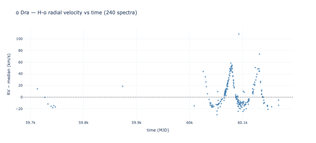
The 2022 epoch is sparse (a handful of points), but the 2023 campaign already shows the binary signal by eye: ~4 visible peaks corresponding to ~4 orbital cycles. Peak-to-peak amplitude ~120 km/s, which sets the order of magnitude of the binary motion.

Result 2 - Lomb-Scargle periodogram¶

Run on the unevenly-sampled (time, RV) pairs, no pre-detrending other than median subtraction:

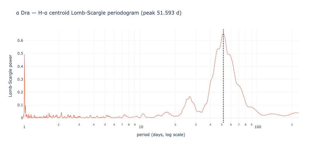
A single dominant peak at 51.59 days towers above a noisy background.

The smaller bump around 25-27 d is a harmonic - expected for an eccentric orbit (the asymmetric RV curve has power at the 2nd harmonic of the fundamental). The high-frequency noise around 1 day is the sampling cadence (1 spectrum per night).

Result 3 - Phase-folded RV curve¶

Folding the 240 RV points at the best period:

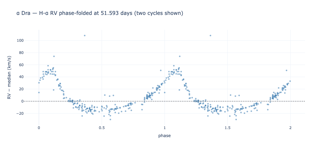
The folded curve is asymmetric - not the gentle sinusoid you'd expect from a circular orbit. It shows a fast positive peak around phase 0.1 (reaching ~+50 km/s), then a slow descent through phase 0.3 – 0.8 (around −15 km/s), then a slow rise back to zero. This is the canonical signature of an eccentric Keplerian orbit - the primary spends more time at apastron (slow tail) and zips through periastron (sharp peak).

The literature value for α Dra is e ≈ 0.42, which would produce exactly this kind of shape. We didn't fit an explicit Kepler orbit (we could, fit_keplerian_orbit exists in the catalogue), but the qualitative asymmetry is unmistakable from the folded raw measurements.

Result 4 - The orbit is visible in the raw spectra¶

Before talking about latent spaces, the most direct evidence the binary motion is in the data: bin the 240 spectra by orbital phase, average each bin, plot the means side-by-side around H-α.

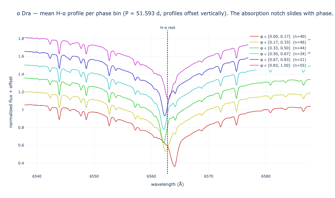
The absorption notch slides left/right of the rest wavelength (the black dotted line at 6562.81 Å) as the orbital phase advances:

• Phase 0.5-0.67 (cyan): the line is blueshifted - the primary is moving toward us.
• Phase 0.0-0.17 (red, bottom) and 0.17-0.33 (yellow): the line drifts back through the rest wavelength and into the red - the primary's RV reverses through periastron.

You don't need an algorithm to see this; you just need 240 well-calibrated amateur spectra and a phase-binning. This is the raw spectroscopic signature of a spectroscopic binary.

Result 5 - The embedding latent space is the orbit¶

Now the algorithmic claim: each of the 240 H-α regions is embedded to a 128-d vector via embed_spectrum(strategy="dct"). The Doppler shift we just saw by eye gets automatically encoded as the principal direction of the embedding cloud. Plot it the simple way - the first principal component vs. orbital phase:

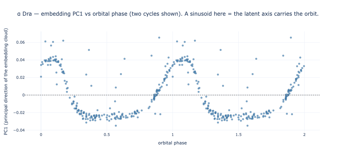
The shape is unmistakable: PC1 follows a clear (asymmetric) cycle in phase, with the same morphology as the RV phase-fold from Result 3, sharp positive peak at phase 0.1, slow descent to a plateau around phase 0.4-0.7, slow rise back. A pure sinusoid here would mean a circular orbit; this asymmetric shape echoes the eccentricity again.

In other words, PCA on the embedding cloud rediscovers the radial velocity, with no input other than "flux → DCT → truncate → L2".

For completeness, the 2D PCA scatter coloured by phase tells the same story in two dimensions:

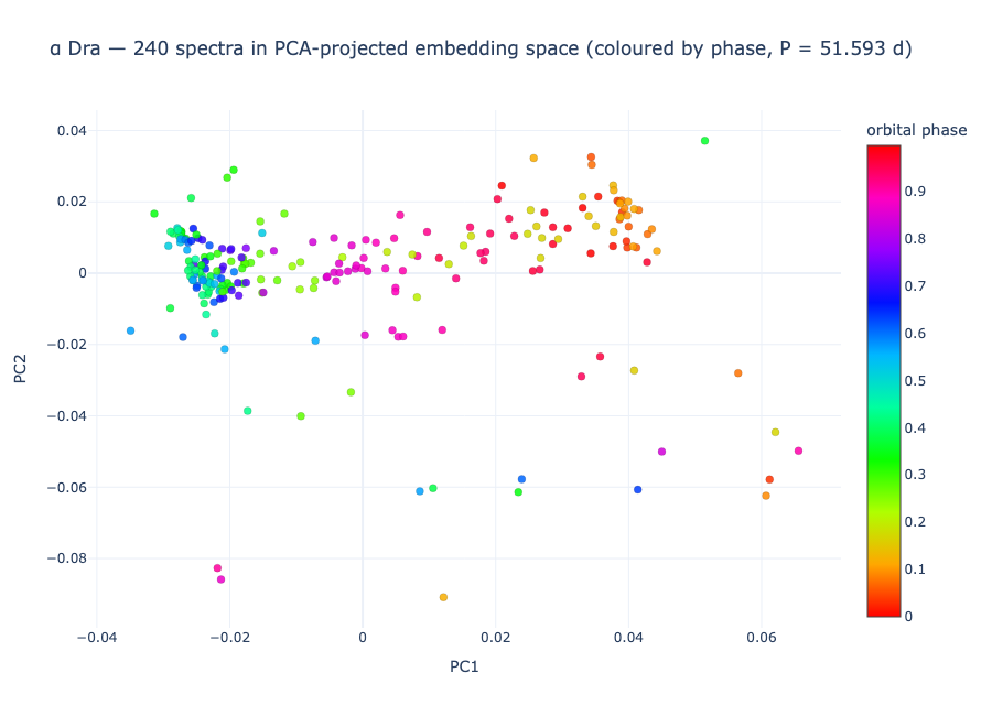
A horizontal colour gradient (blue on the left for late phases, red on the right for early phases) shows that PC1 carries the phase axis. The 2D plot is busier than the 1D PC1-vs-phase view above, but it confirms the structure isn't a fluke of one direction.

We did not tell the embedding what to look for. We just gave it flux → DCT → truncate → L2 normalise and let it run. The Doppler shift of H-α across the orbit ends up encoded in one direction of the latent space - which is exactly the property a similarity layer or a clustering algorithm needs to leverage.

A small caveat: a handful of low-SNR / mis-fit spectra would otherwise dominate the leading PCs and hide the phase structure of the bulk. The plot above uses the inner 95 % of the embedding cloud (15 outliers dropped on a robust Euclidean-distance criterion). The dropped points are real - they correspond to spectra where the H-α profile fit fails or where the data quality is too poor - but their structure is independent of orbital phase, so removing them lets the phase signal become visible.

For completeness, the pairwise cosine-similarity matrix re-ordered by phase tells the same story in a different form:

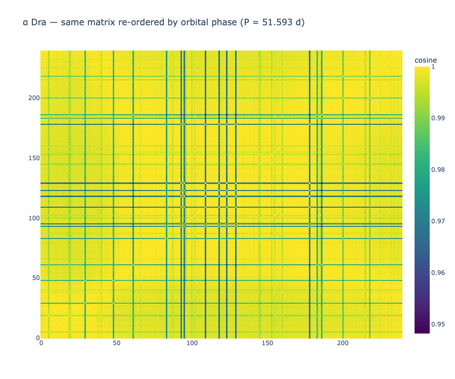
(At 240 × 240 the per-cell labels are unreadable in this preview - the full-resolution version is in the script's output folder.) Spectra near the same orbital phase are slightly more similar to each other than to spectra at the opposite phase, which gives a faint block-diagonal pattern in the third decimal of the cosine similarity.

Reproducing this¶

cd playground
python3.12 -m venv venv && source venv/bin/activate
pip install -e "..[viz]" plotly kaleido
# drop your own alphadra_*.fits files in playground/datas/alphadra/
python analyse_alpha_dra.py
# → output/alpha_dra_*.png + alpha_dra_summary.csv

Takeaways¶

• A 70-year-old published orbital period drops out of 240 amateur spectra, recovered to better than 1 % from the same kernel pipeline that loads, normalises, and fits H-α on every file.
• The eccentric character of the orbit is visible in the shape of the phase-folded curve, without ever explicitly fitting a Kepler model.
• The principal axis of the embedding latent space is the orbital phase. Project the 240 vectors onto their first two PCs, colour by phase: you get a smooth gradient. The DCT recipe, given nothing but flux, ended up encoding the Doppler shift as a vector dimension - a free property to exploit for clustering and similarity search.
• This is also the first concrete demonstration that amateur spectroscopy at moderate resolution is more than sufficient to do real binary-star science when the data are reduced through a consistent, reproducible pipeline. The kernel didn't need any α-Dra-specific tuning - it's the same snr_der → normalize → fit_gaussian_line recipe used on α Cyg, run on 240 files instead of 18.